library(tidyverse)27 A field guide to base R
Introduction
本章介绍一些base R中的重要函数:
- 提取多个元素——
[ - 提取单个元素——
[&$ apply家族for循环- Plot
使用[提取多个元素
提取向量
五种常见情景:
- 正整数表示元素位置提取,重复提取生成重复元素的向量。
x <- c("one", "two", "three", "four", "five")
x[c(3, 2, 5)]
#> [1] "three" "two"   "five"

x[c(1, 1, 5, 5, 5, 2)]
#> [1] "one" "one" "five" "five" "five" "two"- 负整数表示删除对应位置的元素。
x[c(-1, -3, -5)]
#> [1] "two" "four"- 逻辑向量提取值为
TRUE的元素;关于NA的处理与dplyr::filter()不同,前者保留,后者不保留。
x <- c(10, 3, NA, 5, 8, 1, NA)

# All non-missing values of x
x[!is.na(x)]
#> [1] 10  3  5  8  1

# All even (or missing!) values of x
x[x %% 2 == 0]
#> [1] 10 NA 8 NA- 字符串向量提取有name属性的向量元素。
x <- c(abc = 1, def = 2, xyz = 5)
x[c("xyz", "def")]
#> xyz def
#> 5 2- nothing–
x[]返回完整的对象,在后面对data.frame提取时有用。
提取数据框
使用df[rows, cols]提取数据框中对应的行或列;其中rows和cols与上面的使用方法一致。
df <- tibble(
  x = 1:3,
  y = c("a", "e", "f"),
  z = runif(3)
)

# Select first row and second column
df[1, 2]
#> # A tibble: 1 × 1
#>   y
#>   <chr>
#> 1 a

# Select all rows and columns x and y
df[, c("x", "y")]
#> # A tibble: 3 × 2
#>       x y
#>   <int> <chr>
#> 1     1 a
#> 2     2 e
#> 3     3 f

# Select rows where `x` is greater than 1 and all columns
df[df$x > 1, ]
#> # A tibble: 2 × 3
#>       x y         z
#>   <int> <chr> <dbl>
#> 1     2 e     0.834
#> 2 3 f 0.601data.frame格式与tibble格式的数据框在使用[上的唯一区别是:当df[,cols]中的cols只有一个元素时,data.frame格式返回向量,而tibble格式仍返回tibble。
df1 <- data.frame(x = 1:3)
df1[, "x"]
#> [1] 1 2 3

df2 <- tibble(x = 1:3)
df2[, "x"]
#> # A tibble: 3 × 1
#>       x
#>   <int>
#> 1     1
#> 2     2
#> 3 3data.frame格式使用drop参数,可以避免降维。
df1[, "x", drop = FALSE]
#>   x
#> 1 1
#> 2 2
#> 3 3
dplyr 中的等价操作
在dplyr包中有几个verb等价于[的特例:
filter():等价于按行使用逻辑向量提取,但对于NA的处理不同,filter()不保留NA,而[保留。
df <- tibble(
  x = c(2, 3, 1, 1, NA),
  y = letters[1:5],
  z = runif(5)
)
df |> filter(x > 1)
#> # A tibble: 2 × 3
#>       x y           z
#>   <dbl> <chr>   <dbl>
#> 1     2 a     0.157
#> 2     3 b     0.00740

# same as
df[!is.na(df$x) & df$x > 1, ]
#> # A tibble: 2 × 3
#>       x y           z
#>   <dbl> <chr>   <dbl>
#> 1     2 a     0.157
#> 2     3 b     0.00740

df[which(df$x > 1), ]
#> # A tibble: 2 × 3
#>       x y           z
#>   <dbl> <chr>   <dbl>
#> 1     2 a     0.157
#> 2 3 b 0.00740arrange():等价于按行使用正整数向量提取,向量通常由order()生成。
df |> arrange(x, y)
#> # A tibble: 5 × 3
#>       x y           z
#>   <dbl> <chr>   <dbl>
#> 1     1 c     0.466
#> 2     1 d     0.498
#> 3     2 a     0.157
#> 4     3 b     0.00740
#> 5    NA e     0.290

# same as
df[order(df$x, df$y), ]
#> # A tibble: 5 × 3
#>       x y           z
#>   <dbl> <chr>   <dbl>
#> 1     1 c     0.466
#> 2     1 d     0.498
#> 3     2 a     0.157
#> 4     3 b     0.00740
#> 5 NA e 0.290select()&relocate():等价于按列使用字符向量提取。
df |> select(x, z)
#> # A tibble: 5 × 2
#>       x       z
#>   <dbl>   <dbl>
#> 1     2 0.157
#> 2     3 0.00740
#> 3     1 0.466
#> 4     1 0.498
#> 5    NA 0.290

# same as
df[, c("x", "z")]
#> # A tibble: 5 × 2
#>       x       z
#>   <dbl>   <dbl>
#> 1     2 0.157
#> 2     3 0.00740
#> 3     1 0.466
#> 4     1 0.498
#> 5 NA 0.290使用[[和$提取单个元素
Data Frames
[[和$用来提取数据框中的某列;[[可以通过位置或name属性提取,而$只能通过name属性提取。
tb <- tibble(
  x = 1:4,
  y = c(10, 4, 1, 21)
)

# by position
tb[[1]]
#> [1] 1 2 3 4

# by name
tb[["x"]]
#> [1] 1 2 3 4
tb$x
#> [1] 1 2 3 4dplyr包提取了pull()函数,它等价于[[和$。
tb |> pull(x)
#> [1] 1 2 3 4
Tibbles
data.frame与tibble在使用$时有着显著的不同;前者遵循部分匹配原则,后者使用精确匹配原则。
df <- data.frame(x1 = 1)
df$x
#> [1] 1
df$z
#> NULL
tb <- tibble(x1 = 1)
tb$x1
#> [1] 1
tb$z
#> NULLdplyr::mutate的等价操作
下面是使用with(),within()和transform()进行等价操作的例子。
data(diamonds, package = "ggplot2")

# Most straightforward
diamonds$ppc <- diamonds$price / diamonds$carat

# Avoid repeating diamonds
diamonds$ppc <- with(diamonds, price / carat)

# The inspiration for dplyr's mutate
diamonds <- transform(diamonds, ppc = price / carat)
diamonds <- diamonds |> transform(ppc = price / carat)

# Similar to transform(), but uses assignment rather argument matching
# (can also use = here, since = is equivalent to <- outside of a function call)
diamonds <- within(diamonds, {
  ppc <- price / carat
})
diamonds <- diamonds |> within({
  ppc <- price / carat
})

# Protect against partial matching
diamonds$ppc <- diamonds[["price"]] / diamonds[["carat"]]
diamonds$ppc <- diamonds[, "price"] / diamonds[, "carat"]

# FORBIDDEN
attach(diamonds)
diamonds$ppc <- price / carat
lists
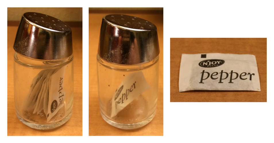
[,[[和$都可以提取list中的元素,但[保留原list层级,而[[和$不保留。
l <- list(
  a = 1:3,
  b = "a string",
  c = pi,
  d = list(-1, -5)
)

str(l[1:2])
#> List of 2
#>  $ a: int [1:3] 1 2 3
#>  $ b: chr "a string"

str(l[1])
#> List of 1
#>  $ a: int [1:3] 1 2 3
str(l[[1]])
#>  int [1:3] 1 2 3

str(l[4])
#> List of 1
#>  $ d:List of 2
#>   ..$ : num -1
#>   ..$ : num -5
str(l[[4]])
#> List of 2
#>  $ : num -1
#>  $ : num -5
两者的差异如下图所示:
Apply 家族
在apply家族中与前章中的map类似的函数是lapply()系,主要针对的是list;而其他如apply()针对array或matrix,tapply()类似group_by()+summarize()。
lapply()系包含lapply()、sapply()、vapply();sapply()函数中的参数simplify可以将结果整理为向量或矩阵,当simplify = FLASE时与lapply()等价;vapply()函数与sapply()相同但更严格,一定会simplify为向量或矩阵,同时必须通过参数FUN.VALUE提供返回值的类型。下面是一些示例:
x <- list(a = 1:10, beta = exp(-3:3), logic = c(TRUE, FALSE, FALSE, TRUE))
# compute the list mean for each list element
lapply(x, mean)
#> $a
#> [1] 5.5
#>
#> $beta
#> [1] 4.535125
#>
#> $logic
#> [1] 0.5
# median and quartiles for each list element
lapply(x, quantile, probs = 1:3 / 4)
#> $a
#>  25%  50%  75%
#> 3.25 5.50 7.75
#>
#> $beta
#>       25%       50%       75%
#> 0.2516074 1.0000000 5.0536690
#>
#> $logic
#> 25% 50% 75%
#> 0.0 0.5 1.0
sapply(x, quantile)
#>          a        beta logic
#> 0%    1.00  0.04978707   0.0
#> 25%   3.25  0.25160736   0.0
#> 50%   5.50  1.00000000   0.5
#> 75%   7.75  5.05366896   1.0
#> 100% 10.00 20.08553692   1.0
i39 <- sapply(3:9, seq) # list of vectors
sapply(i39, fivenum)
#>      [,1] [,2] [,3] [,4] [,5] [,6] [,7]
#> [1,]  1.0  1.0    1  1.0  1.0  1.0    1
#> [2,]  1.5  1.5    2  2.0  2.5  2.5    3
#> [3,]  2.0  2.5    3  3.5  4.0  4.5    5
#> [4,]  2.5  3.5    4  5.0  5.5  6.5    7
#> [5,]  3.0  4.0    5  6.0  7.0  8.0    9
vapply(
  i39, fivenum,
  c(Min. = 0, "1st Qu." = 0, Median = 0, "3rd Qu." = 0, Max. = 0)
)
#>         [,1] [,2] [,3] [,4] [,5] [,6] [,7]
#> Min.     1.0  1.0    1  1.0  1.0  1.0    1
#> 1st Qu.  1.5  1.5    2  2.0  2.5  2.5    3
#> Median   2.0  2.5    3  3.5  4.0  4.5    5
#> 3rd Qu.  2.5  3.5    4  5.0  5.5  6.5    7
#> Max. 3.0 4.0 5 6.0 7.0 8.0 9apply()在处理非array或matrix时,会首先执行as.array()或as.matrix()。所以apply(df, 2, something)这种方法一定要慎用,相较于lapply(df, something),它更缓慢且具有隐藏风险。
tapply()函数与group_by()+summarize()等价,但tapply()返回的是向量。
diamonds |>
  group_by(cut) |>
  summarize(price = mean(price))
#> # A tibble: 5 × 2
#>   cut       price
#>   <ord>     <dbl>
#> 1 Fair      4359.
#> 2 Good      3929.
#> 3 Very Good 3982.
#> 4 Premium   4584.
#> 5 Ideal     3458.

tapply(diamonds$price, diamonds$cut, mean)
#>      Fair      Good Very Good   Premium     Ideal
#>  4358.758  3928.864  3981.760  4584.258  3457.542
for Loops
for 循环的基本格式如下:
for (element in vector) {
  # do something with element
}
for 循环在R中十分常用,但是我们要避免下面格式的循环,不断地对环境变量进行赋值修改:
out <- NULL
for (path in paths) {
  out <- rbind(out, readxl::read_excel(path))
}本文提供了另外一种标准地书写格式:先创建固定长度地list,然后使用do.call()函数将list中的元素进行拼接。
files <- vector("list", length(paths))
seq_along(paths)
#>  [1]  1  2  3  4  5  6  7  8  9 10 11 12
for (i in seq_along(paths)) {
  files[[i]] <- readxl::read_excel(paths[[i]])
}
do.call(rbind, files)
#> # A tibble: 1,704 × 5
#>   country     continent lifeExp      pop gdpPercap
#>   <chr>       <chr>       <dbl>    <dbl>     <dbl>
#> 1 Afghanistan Asia         28.8  8425333      779.
#> 2 Albania     Europe       55.2  1282697     1601.
#> 3 Algeria     Africa       43.1  9279525     2449.
#> 4 Angola      Africa       30.0  4232095     3521.
#> 5 Argentina   Americas     62.5 17876956     5911.
#> 6 Australia   Oceania      69.1  8691212    10040.
#> # ℹ 1,698 more rows
Plots
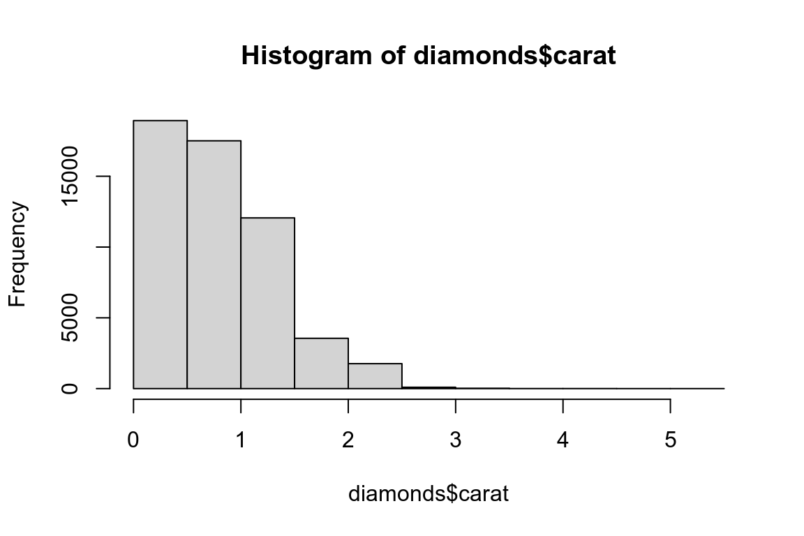
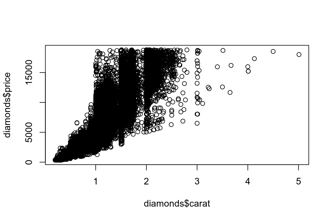
虽然ggplot2是一个强大的绘图工具,但是baseR中的一些函数在数据分析探索阶段使用起来十分便利,例如plot和hist。
# Left
hist(diamonds$carat)

# Right
plot(diamonds$carat, diamonds$price)